Animation More Better
A short vignette on understanding advanced gganimate features and how they can improve your animated data visualisations


- Author
- Joshua McCarthy
- Published
- Sat, Feb 22 2020
- Last Updated
- Sat, Feb 22 2020
#Load required libraries
library("tidyverse")
library("gganimate")
library("gifski")
Intro
Animating a plot is an engaging way to communicate information. A simple animation blends the transition from the starting state to the end state with a constant motion. However, our understanding of what makes interesting, appealing and effective animated motion has developed over the years as the complexity of the motion has increased. It is now common to see high quality animation every day in our digital lives, in actions as simple as mousing over a menu button, to the point where it is often more jarring to see poor motion than excellent. To avoid this, this how we make our animations in R ‘More Better’! (using gganimate)
See an excellent intro to animation using gganimate from Joe Drigo Enriquez here.
Setup & Understanding
First, we create some simple plots.
#Create sample data frame
simple_point <- data.frame(ball = 1, time = seq(from = 0, to = 200, by = 50))

#plot of data frame
ggplot(simple_point, aes(x=time, y=ball, group = ball)) + geom_point(size = 4)
Simple Plot
#Sine wave
sine <- data.frame(timer =  seq(from = 0, to =9.9, by = 0.1))
ggplot (sine, aes(x = timer)) + geom_line(aes(y = sin(timer)))
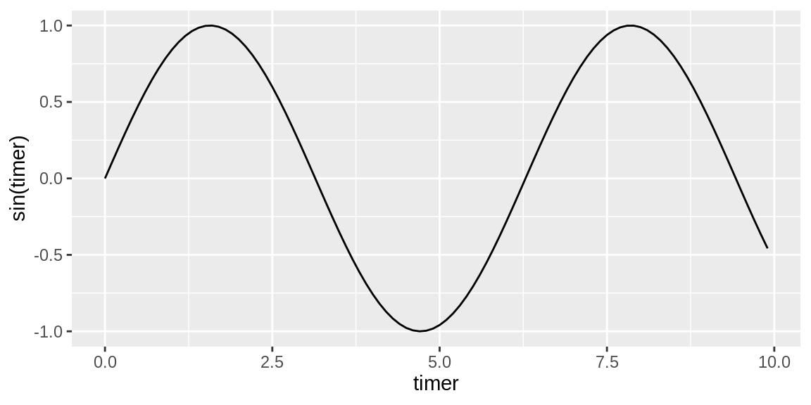
Simple Sine Plot
Now a simple animation of the plot, it is not necessary to assign the plot and then call the animate function, however this overcomes some inconsistencies with sizing of the plot in Rmarkdown. This animation uses all default settings.
#creating animation based on time
simple_anim <- ggplot(simple_point, aes(x=time, y=ball, group = ball)) + geom_point(size = 4) +
  transition_states(time, wrap = FALSE) #ggplot code to animate over variable in data frame "time"

simple_sine <- ggplot (sine, aes(x = timer)) + geom_line(aes(y = sin(timer))) +
  transition_reveal(timer)

#calling animate function to render animation
animate(simple_anim)

Simple Animation
animate(simple_sine)

Simple Sine Animation
States & Keyframes
Gganimate utilises the transition_ function to control the animation. ‘Transition_states’ uses states, which are similar to keyframes used in animation. States define what is included in a snapshot of the plot, the transition motion is then interpolated from one snapshot to the next. The transition time will be the same from one state to the next regardless of how much the variable changes even for continuous variables. This transition time is set with transition_length. The animation will then pause at each state for a time set by state_length. For our above plot, to smooth the motion we need to either set state_length to 0 (similar to if transition_time was used), or only apply a state to the first and last observation.
simple_point_state <- simple_point
simple_point_state$state <- NA #create a variable to set states

#Define each state we wish to transition between
simple_point_state[1,3] <- 1
simple_point_state[5,3] <- 2

#na.omit can be used to remove uneeded data
simple_anim_state <- ggplot(na.omit(simple_point_state), aes(x=time, y=ball, group = ball)) + geom_point(size = 4) +
  transition_states(state, wrap = FALSE) #ggplot code to animate over variable in data frame "time"

animate(simple_anim_state)

Animation with States
Frame Rate
The simplest improvement we can make is to modify the framerate. The default framerate for gganimate is 10FPS (Frames per second), generally the minimum framerate for smooth motion is 30FPS
animate(simple_anim_state, nframes= 105, fps = 30)

30fps Animation
That’s quite a bit better, we can up it to a max of 50fps, 60fps would be ideal but this is not supported by gganimate and gifski. Note in order to maintain a consistent animation time the number of frames must equal animation length * fps. The drawback being that animations with more frames take longer to process.
animate(simple_anim_state, nframes= 175, fps = 50)

50fps Animation
animate(simple_sine, nframes = 175, fps = 50)
50fps Sine Animation
Pauses
People require time to understand what the visualisation is showing (e.g. title, axis labels, scale) and what the final image means, the more complexity displayed the longer needed to absorb, we can modify the pauses between loops as below. A similar principle must be applied to the time at each state once the transition has been made, set using the state_legnth function as mentioned previously.
#pauses are set in frames, and are included in the total number of frames, nframes will need to modified accordingly
animate(simple_anim_state, nframes= 175, fps = 50, start_pause = 50, end_pause = 50)

Paused Animation
Easing
Smoother movement has highlighted one of the major drawbacks of simple motion, the current animation has a constant motion, or velocity throughout the transition, described as ‘linear’ easing, which is quite unnatural. Compare this motion with the following animations.
impr_anim_state <- ggplot(na.omit(simple_point_state), aes(x=time, y=ball, group = ball)) + geom_point(size = 4) +
  transition_states(state, wrap = FALSE) +
  ease_aes("quintic-in-out")

animate(impr_anim_state, nframes= 200, fps = 50)

Eased Animation
A much more natural motion. Ease functions control the velocity of the elements during the transition, linear easing representing a straight line or constant velocity, other easing functions represent a curve, higher functions have a smaller ‘radius’ meaning the velocity changes faster, in order of rate of change; quadratic, cubic, quartic and quintic.
More ease functions can be found here and easily visualised here however these more complex movements can be more of a distraction than an aid.
Quadratic has the slowest rate of change
impr_anim_state <- ggplot(na.omit(simple_point_state), aes(x=time, y=ball, group = ball)) + geom_point(size = 4) +
  transition_states(time, wrap = FALSE) +
  ease_aes("quadratic-in-out")

animate(impr_anim_state, nframes= 200, fps = 50)

Quadratic Easing
Quintic has the fastest rate of change
impr_anim_state <- ggplot(na.omit(simple_point_state), aes(x=time, y=ball, group = ball)) + geom_point(size = 4) +
  transition_states(time, wrap = FALSE) +
  ease_aes("quintic-in-out")

animate(impr_anim_state, nframes= 200, fps = 50)

Quintic Easing
Bounce introducing an unrealistic representation of the data.
impr_anim_state <- ggplot(na.omit(simple_point_state), aes(x=time, y=ball, group = ball)) + geom_point(size = 4) +
  transition_states(time, wrap = FALSE) +
  ease_aes("bounce-out")

animate(impr_anim_state, nframes= 200, fps = 50)

Bouncer
Though it can be somewhat commical
impr_anim_state <- ggplot(na.omit(simple_point_state), aes(x=ball, y=time, group = ball)) + geom_point(size = 10) + scale_y_reverse() +
  transition_states(time, wrap = FALSE) +
  ease_aes("bounce-out") +
  labs(title = "Doomed", x = "bottom", y = "price")

animate(impr_anim_state, nframes= 200, fps = 50)

Oh Dear
OH NO! IT’S HIT ROCK BOTTOM!
##Types of ease
This figure highlights another variation of ease, most plots shown have utilise in-out ease functions, where bounce was applied as an out function, the three variations of ease are;
Ease-in - The curve starts at 0 velocity and increases throughout the animation
impr_anim_state <- ggplot(na.omit(simple_point_state), aes(x=time, y=ball, group = ball)) + geom_point(size = 4) +
  transition_states(time, wrap = FALSE) +
  ease_aes("quintic-in")

animate(impr_anim_state, nframes= 200, fps = 50)

Ease-in
Ease-out - The curve starts at peak velocity and decreases to 0 throughout the animation
impr_anim_state <- ggplot(na.omit(simple_point_state), aes(x=time, y=ball, group = ball)) + geom_point(size = 4) +
  transition_states(time, wrap = FALSE) +
  ease_aes("quintic-out")

animate(impr_anim_state, nframes= 200, fps = 50)

Ease-out
Ease-in-out - Represents a parabola starting at 0 increasing to a peak at the median of the transition and decreasing back to 0 at the end.
impr_anim_state <- ggplot(na.omit(simple_point_state), aes(x=time, y=ball, group = ball)) + geom_point(size = 4) +
  transition_states(time, wrap = FALSE) +
  ease_aes("quintic-in-out")

animate(impr_anim_state, nframes= 200, fps = 50)
Ease-in-out
Additonal uses
Ease can be use creatively to improve comprehension of your visualisation, though tread carefully, ease can be misleading. See the below examples.
Ease-in can create a sense of urgency and the perception the data continues on
e_in <- data.frame(a=c(1,2), b=c(1,2))

e_in_anim <- ggplot(e_in, aes(x=b, y=a)) + geom_line() +
  transition_reveal(b, keep_last = TRUE) +
  ease_aes("exponential-in")

animate(e_in_anim, nframes= 200, fps = 50, end_pause = 100)
Urgent Plot
Ease-out gives the perception that the change is slowing down
e_out <- data.frame(a=c(1,2), b=c(2,1))

e_out_anim <- ggplot(e_out, aes(x=a, y=b)) + geom_line() +
  transition_reveal(a, keep_last = TRUE) +
  ease_aes("exponential-out")

animate(e_out_anim, nframes= 250, fps = 50, end_pause = 100)

Shutting Down Plot
Ease-in-out implies the analysis only occurs within a certain range
e_in_out <- data.frame(a=c(1,2), b=c(1,1))

e_in_out_anim <- ggplot(e_in_out, aes(x=a, y=b)) + geom_line() +
  transition_reveal(a, keep_last = TRUE) +
  ease_aes("quintic-in-out")

animate(e_in_out_anim, nframes= 300, fps = 50, end_pause = 100)
Closed Plot
Ease-in-out also does quite a good job of highlighting each state the animation moves through
e_in_out_anim2 <- ggplot(simple_point, aes(x=time, y=ball, group = ball)) + geom_point(size = 4) +
  transition_states(time) +
  ease_aes("quintic-in-out")

animate(e_in_out_anim2, nframes= 300, fps = 50)

Stepped Plot
Duration
Finally, we have nice smooth natural motion, the final consideration covered in this vignette is keeping people’s attention. The duration of the animation needs to find a balance between being too fast for ease of comprehension and too slow so as to lose the observer’s attention. Google gives examples of common speeds here in the material design guide ~300ms. in the material design guide ~300ms. The ubiquity of these transition speeds in every day digital life mean that deviating from this can result in a poor impression.
animate(impr_anim_state, nframes= 45, fps = 50)

Snappy Duration
If your animation is moving through multiple states, consider the duration as the time between each state. If your animation has five states including beginning and end, while being equally complex as an animation with two states it would have the same duration between each state as the whole of the two state animation, resulting in an animation four times as long.
e_in_out_anim_dur<- ggplot(simple_point, aes(x=time, y=ball, group = ball)) + geom_point(size = 4) +
  transition_states(time) +
  ease_aes("quintic-in-out")

animate(e_in_out_anim_dur, nframes= 225, fps = 50)

Stepped Snappy Duration
When the scale of the transition is important, it can be useful to increase or decrease the transition duration accordingly to communicate the magnitude, similar considerations can be used based on element size.
big_point_state <- data.frame(sun = 1, time = seq(from = 0, to = 200000, by = 50000))
big_point_state$state <- NA
big_point_state[1,3] <- 1
big_point_state[5,3] <- 2

big_anim_state <- ggplot(na.omit(big_point_state), aes(x=time, y=sun, group = sun)) + geom_point(size = 36) +
  transition_states(state, wrap = FALSE)

animate(big_anim_state, nframes= 900, fps = 50)
Big Plot
Conclusion
Animation has undergone significant refinement over the years, by drawing on this existing understanding and applying it to how we present our visualisations we can relatively easily increase the appeal, engagement and comprehension of our analysis. Best of luck and make your plots more better!